ARCHIVE
Vol. 5, No. 1
JANUARY-JUNE, 2015
Research Articles
Special Essay
Field Reports
Discussion
Book Reviews
Spatial Characteristics of Long-Term Changes in
Indian Agricultural Production:
District-Level Analysis, 1965-2007
Takashi Kurosaki* and Kazuya Wada†
*Institute of Economic Research, Hitotsubashi University, Tokyo, kurosaki@ier.hit-u.ac.jp
†Faculty of Global Communication, University of Nagasaki, Nagayo-cho
Abstract: In this paper, we comprehensively describe spatial patterns of long-term changes in Indian agriculture at the district level. Variables of concern include the intensity of land-use, the shares of rice and wheat in areas under foodgrains, the ratio of non-foodgrains in gross cultivated area, the intensity of fertilizer-use, and individual crop shares in gross cultivated areas. As one outcome of the descriptive analysis, we propose a new regional classification of Indian districts based on similarity in rainfall, initial cropping and land-use patterns, and initial conditions and changes in irrigation. The proposed classification has reasonable explanatory power in describing the spatial patterns of long-term changes at the district level.
Keywords: Spatial resource allocation, land-use intensity, crop mix, India.
1. Introduction
Sustaining agricultural growth is key to rural development and poverty reduction in India. As the room for extensive expansion has almost disappeared in Indian agriculture, it is critically important to improve land productivity to sustain growth. Among the various factors that contribute to productivity improvement, the introduction of new technology has been investigated most intensively in the literature. For example, in the standard literature on long-term growth in agricultural production in India, the contribution of the Green Revolution that began in the late 1960s has been emphasised (e.g., Bhalla and Tyagi 1989, Bhalla and Singh 2001, Bhalla and Singh 2009, Bhalla and Singh 2012). Green Revolution technology is characterised by high-yielding seeds, chemical fertilizer, and irrigation. Another area on which the existing literature has focused — as shown in the pages of the Review of Agrarian Studies — is that of institutions, including land tenancy, labour market institutions, and credit markets.
Besides these, there is another source of agricultural productivity growth, one less investigated in the literature. Even with little improvement in per-acre yield of individual crops, the productivity of land can increase through the reallocation of crops from low value-added to high value-added crops and from regions where productivity is low to regions where productivity is high. Using a longer-term horizon than adopted in the traditional literature, Kurosaki (2002, 2011, 2015) showed that sustained growth in agricultural production began in India during the 1950s, much earlier than the onset of the Green Revolution, and shifts from low- to high-value crops (changes in cropping patterns) contributed to agricultural growth during the earlier growth period. Similar findings were obtained for areas currently in Pakistan Punjab (Kurosaki 2003). Kurosaki (2003) also demonstrated that crop shifts from low-productivity districts to high-productivity districts contributed to agricultural growth in West Punjab, especially during the colonial period. Nevertheless, there is a dearth of empirical studies on the contribution of spatial crop shifts to productivity improvement in post-Independence Indian agriculture.
This paper describes spatial patterns of long-term changes in Indian agriculture at the district level for the period from 1965 to 2007. The analysis employs the district, as defined by district boundaries prevalent in 1965, as the unit of investigation. The paper is descriptive in nature, and does not aim to rigorously investigate the role of technology or policies or agrarian structure. Which districts produced which crops? How have such spatial patterns changed over time? We address these questions in this paper by combining various quantitative methods to describe spatial changes.
Such descriptive information is useful in addressing more fundamental questions, such as those concerning the kinds of market and technology development that characterise Indian agriculture. To understand the salience of such information, a microeconomic theory of spatial equilibrium (Takayama and Judge 1971) is useful. Agricultural production is linked with consumption demand in general. This linkage implies that when agricultural output markets are underdeveloped, farmers in a village produce what people in the village want to consume. This is a situation in which spatial equilibrium is closed within a village as a unit. The equilibrium is characterised by village-specific shadow prices,1 which may diverge from market prices. Without technical innovation in the production of individual crops, there is no room for productivity improvement in this situation. As agricultural output and factor markets develop, however, farmers and villages become more able to respond to demand from outside the village. By shifting to crops whose value added is higher if calculated using market prices, production value can be improved even without innovation in individual crop production technology. If such market development is accompanied by irrigation development, the room for individual farmers to respond to market incentive becomes larger. The spatial pattern of agricultural production changes over time reflects such market and technology development (Takayama and Judge 1971, Timmer 1997).
With this theoretical background, Kurosaki (2003) provided district-level analysis for the case of West Punjab (now in Pakistan) agriculture for the period from 1903 to 1992. This paper shares the research motivation of Kurosaki (2003) but extends the analysis to the whole of India. As all-India district-level analyses of agricultural production, Bhalla and Singh (2001) and Bhalla and Singh (2012) are notable studies. These studies, however, do not interpret the observed spatial changes in the microeconomic framework of market development and spatial equilibrium. Such a focus distinguishes this paper from those studies.
The rest of the paper is organised as follows. Section 2 explains the data used and shows the heterogeneity observed across districts with respect to agricultural intensification. The evidence on heterogeneity is the first descriptive exercise on spatial characteristics of changes in Indian agriculture. As the second descriptive exercise, Section 3 shows district-level GIS maps, which enables an eyeball perusal of changes in spatial production patterns that occurred between 1965 and 2007. In Section 4, we propose new agricultural zones derived from cluster analysis using the district-level data, which is another way to aggregate spatial changes in descriptive analysis. Section 5 adopts a more parametric approach to describe spatial changes, i.e., a regression analysis applied to district-level panel data. The regression analysis identifies correlates of changes in intensification measures. Section 6 presents our conclusions.
2. Data
2.1 Dataset Used
We use the district-level study (DLS) database compiled by the International Crops Research Institute for the Semi-Arid Tropics (ICRISAT). The original data sources include government statistics such as Agricultural Statistics of India and related publications at the State level. The compilation procedure is reported in the DLS manual (ICRISAT 1998). Although our dataset is based on the revised version up to 2007, the DLS manual has not been revised. The period of analysis is 42 years: from agricultural year 1965-6 to agricultural year 2006-7.2 Smaller districts, where agricultural production is negligible and statistics are reported only sporadically, have been dropped from the analysis. Several observations with inconsistent data have also been dropped.
As a result, we employ a balanced panel dataset of 311 districts spread over 19 major States of India (Andhra Pradesh, Assam, Bihar, Chhattisgarh, Gujarat, Haryana, Himachal Pradesh, Jharkhand, Karnataka, Kerala, Madhya Pradesh, Maharashtra, Orissa, Punjab, Rajasthan, Tamil Nadu, Uttar Pradesh, Uttarakhand, and West Bengal) over the 42 years. The 311 districts were based on district borders in 1965. The boundaries of these 311 districts covered 498 districts in 2007. Regarding the State coverage, the analysis excludes 9 small States, including Jammu & Kashmir, Sikkim, and Goa, and 7 federal territories. Figure 1 shows the spatial coverage of these 311 districts.
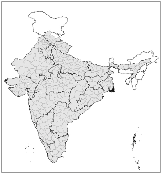
Figure 1 Spatial distribution of the 311 districts analysed
Note: The shaded area within thin lines corresponds to a district (boundaries in 1965) included in this study. Bolder lines show state boundaries in 2014.
Source: Drawn by the authors using the DLS database compiled by ICRISAT.
From the DLS database, we compiled the following variables for analysis. As production factors, we employ gross cultivated area (gca), net cultivated area (nca), irrigation ratio (“net cultivated area, irrigated” divided by nca), quantity of fertilizer (the sum of N, P, and K fertilizers), the number of agricultural markets, the length of paved roads, and rainfall indicators. For individual crops, we employ area and output quantity of rice, wheat, maize, sorghum (jowar), pearl millet (bajra), finger millet (ragi), barley, chickpea (gram), pigeonpea (toor or arhar), and other pulses. The sum of areas under these crops covers 60 to 70 per cent of the gross cultivated area.3
As demonstrated by Kurosaki (2011) and Kurosaki (2015), twentieth-century Indian agriculture can be characterised by sustained growth through improving land productivity and shifts to higher value-added crops. These papers have shown that the index of land use intensity (=gca/nca), the share of rice and wheat in the area under foodgrain crops (srw), and the share of non-foodgrain crops in the gross cultivated area (snfg) gradually increased throughout the century.
2.2 Spatial Heterogeneity in Agricultural Intensification
Has the increase in these measures in agricultural intensification occurred homogeneously in all districts in India? As the first descriptive analysis of spatial characteristics, we plot the district-level trends of gca, intensity, snfg, and srw in a histogram (Figure 2).
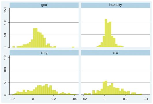
Figure 2 Distribution of average annual growth rates at the district level, 1965-6–2006-7
Note: We first regress a time series model for each of the 311 districts, using the natural logarithm of gca, intensity, snfg, or srw as the dependent variable and the annual trend as the explanatory variable (gca = gross cultivated area, intensity = gca/net cultivated area, snfg = the share of non-foodgrain crops in gca, srw = share of rice and wheat in the areas under foodgrain crops). We then plot the distribution of the 311 parameter estimates in a histogram. To make histograms easy to compare, we trim the range between -.02 (annual average decline at 2 per cent) and .04 (annual average increases at 4 per cent). The number of outliers outside the range is 2 for gca, 0 for intensity, 22 for snfg, and 10 for srw.
Source: Drawn by the authors using the DLS database compiled by ICRISAT.
Figure 2 clearly shows substantial inter-district heterogeneity. Although the four indices were associated with positive trends at the all-India level, the trend was negative for a non-negligible number of districts. Heterogeneity was more substantial for snfg and srw than for gca and intensity. This suggests that, throughout India, gross cultivated area increased, mostly through rising intensity of land use, while the list of crops that occupied the increased area under cultivation differed from district to district. Furthermore, the heterogeneity of trends in snfg and srw has been increasing in recent years.4 In the next section, we examine which crops specifically were responsible for such heterogeneity.
3. Spatial Changes in Agricultural Production, Described through GIS Maps
In this section, we describe spatial changes in agricultural production using GIS maps at the district level. In other words, this is an eyeball investigation of spatial patterns. Each map in the Appendix shows four figures for each variable of interest. The upper left figure plots the initial distribution in five quantiles, where the initial period refers to the three-year average from 1965-6 to 1967-8. The upper right figure (terminal, A) plots the terminal distribution in five quantiles, whose quantile thresholds are the same as those used for the initial quantiles. The terminal period refers to the three-year average from 2004-6 to 2006-7. The lower left figure (terminal, B) plots the terminal distribution in five quantiles, whose quantiles are re-defined over the terminal values. The comparison of the initial and terminal A tells us about absolute changes in spatial patterns, while the comparison of the initial and terminal B tells us about relative changes in spatial patterns. The lower right figure plots the distribution of growth rate. The growth rate was estimated for each district from 42-year data using OLS. We include maps that show interesting spatial changes in the Appendix. Maps not shown in the Appendix are available on request from the authors.
3.1 Cropped Area
Gross cultivated area (gca) increased in most districts in India (Appendix Map 1). The positive trend was more significant in northern districts such as those in Rajasthan, Punjab, Haryana, Madhya Pradesh, West Bengal, and Assam than elsewhere. On the other hand, several districts were associated with negative trends in gca, many of which are in Himachal Pradesh, Bihar, and Tamil Nadu.
Looking at individual crops, rice-dominated districts in the initial years remained mostly the same in the terminal years (Appendix Map 2). Districts with higher trends in rice area than other districts were concentrated in Punjab, Haryana, Chhattisgarh, and West Bengal. Other than the districts in West Bengal, these districts were located inland. Districts with negative trends in rice area were found in Tamil Nadu, Bihar, Jharkhand, and several places in western India.
Wheat production is concentrated in north India (Appendix Map 3), spanning districts in Punjab and Haryana (henceforth called “Punjab region”) to districts in Uttar Pradesh, Bihar, Rajasthan, Madhya Pradesh, and Maharashtra. Districts with higher trends than the national average were also concentrated in the same States, with the exception of Maharashtra. In Maharashtra, districts once cropped with large areas of wheat were associated with negative trends in wheat area, as was the case in districts in south India, where wheat was not much cultivated as part of traditional farming systems.
A distinct spatial contrast is observed with respect to coarse millets. In the case of maize (Appendix Map 4), initial production was concentrated in the northern districts of Punjab, Haryana, Uttar Pradesh, Bihar, Jharkhand, and Rajasthan. In most of these districts, maize area decreased after the mid-1960s. New maize-producing centres have been emerging in Maharashtra, Madhya Pradesh, Karnataka, interior Andhra Pradesh, and interior Tamil Nadu. The production of sorghum (jowar) decreased in most districts throughout India, with no significant change in production centres in districts south of Maharashtra (Appendix Map 5). The production of pearl millet (bajra) also decreased in the majority of districts in India (Appendix Map 6). It is noteworthy that we found several exceptional districts in eastern Rajasthan where bajra area had been increasing. The overall decline was observed for ragi area as well, including those districts — for example, in Tamil Nadu, Karnataka, Andhra Pradesh, and Orissa — where finger millet was once one of the most important crops (Appendix Map 7). In contrast to the overall declining trend, districts in Uttarakhand showed an increase in ragi area. Barley has become a minor crop in most districts, including districts in Uttar Pradesh where barley once occupied a substantial share of the cropped area.
A significant spatial shift of production centres was observed for chickpea (Appendix Map 8). The traditional production centres in northern districts in Punjab, Haryana, Uttar Pradesh, and Bihar witnessed a rapid decline of area under chickpea. New chickpea production districts appeared in Madhya Pradesh, Maharashtra, and northern Karnataka. In other words, the production centre of chickpea has travelled south. Traditional chickpea-producing districts in Uttar Pradesh, Maharashtra, and Karnataka experienced a slight decrease in area under the crop. No new centre of significance is emerging, however. The production of other pulses is, on average, on the decline other than in several districts in Orissa.
3.2 Intensity of Land Use
As summary measures of cropping patterns focusing on the change in land use intensity, Appendix Maps 9–11 plot intensity, srw, and snfg, which were already discussed in Figure 2 regarding the heterogeneity among districts. By looking at the maps, we can pinpoint the places where each of these measures increased or decreased.
The variable intensity was high in the initial years (the 1960s) in districts located in Punjab, Uttar Pradesh, Orissa, and West Bengal (Appendix Map 9). This regional pattern remained the same in terminal years during the 2000s. Trends in intensity were positive in the majority of districts, especially in those districts whose initial level of intensity was high. Districts associated with a decline in intensity were concentrated in Tamil Nadu and Himachal Pradesh.
The importance of rice and wheat in foodgrain production (srw) was high in initial years in districts located in the Punjab region, Uttar Pradesh, West Bengal, western Orissa, and coastal districts on the Arabian Sea (Appendix Map 10). The trends in srw were highly positive in the Punjab region and Uttar Pradesh, and negative in Orissa. Changes in cropping patterns in the direction of Green Revolution crops occurred more in the Punjab region than elsewhere. Furthermore, many arid districts in Rajasthan, where rice or wheat were not cultivated due to the lack of water, experienced a rapid increase in srw, thanks to recent irrigation development. In northern and western parts of India, irrigation in arid and semi-arid environments clearly favoured these Green Revolution crops.
The tendency to grow pure cash crops is captured by the variable snfg (Appendix Map 11). In initial years, snfg was high in the western half of India, coming down from Punjab in the north to Tamil Nadu and Kerala in the south. As trends in snfg were lower in Punjab than in the western and southern parts of India, snfg became higher in the western and southern parts of India but not in north-western India in the terminal years. In other words, the spatial change in cropping patterns was heterogeneous across regions, reflecting the differing comparative advantage of each district with respect to different crops. In some districts, the direction of change was towards Green Revolution crops, while in others the direction was away from Green Revolution crops.
3.3 Interpretation
The descriptive analysis in this section implies the following. First, regarding the area under crops, Indian agriculture reached the limits of extensive expansion in the late nineteenth and early twentieth centuries (Kurosaki 2015). To overcome the limits on expansion through extensive growth, land use intensity increased, especially in north India, where irrigation developed. The spread of chemical fertilizer was another factor that contributed to the intensification of land use, but the spread was also facilitated by irrigation. During the initial years of our reference period, irrigation was better developed in north India and districts on the Bay of Bengal coast, including districts of Tamil Nadu. Water availability improved almost everywhere since then. The districts that experienced higher growth in land intensity overlapped with districts where irrigation developed relatively fast.
Throughout the reference period of our analysis, we observed shifts in cropping patterns, for example, an increase in the area under rice and wheat in the Punjab region, and new production centres with respect to millets in the interior parts of India. These changes suggest that production specialisation has been going on in response to comparative advantages associated with heterogeneous climatic conditions and irrigation development. As Kurosaki (2003) suggested, rural infrastructure such as roads and markets could be responsible for these changes as well. According to the same study, there were two different phases of development of agricultural output markets. The first, which involved local market integration linking nearby villages and cities, occurred during the colonial period, and the second, characterised by national market integration, occurred after Independence in 1947. The spatial changes observed during the period of our study suggest that the process continued in independent India.
4. A New Typology of Indian Agriculture
4.1 Empirical Strategy: Cluster Analysis Using District-Level Data
In the previous section, spatial changes observed in GIS maps were discussed using States as the main unit of regional variation within India. However, in many cases, within-State heterogeneity is significant, and, in other cases, some districts in a State showed patterns more similar to districts in the neighbouring State than to the other districts in the same State. Using zones of regional typology is thus a convenient tool to aggregate spatial changes in descriptive analysis.
In the literature, several typologies of regional zones with respect to Indian agriculture have been proposed. They include State boundaries, as used in Section 3; fifteen agro-climatic zones designated by the Indian Ministry of Agriculture; agro-climatic regions from B1 to B8 of the ICRISAT, which were employed in ICRISAT (1998); a more recent attempt at ICRISAT (Rao et al. 2004), discussed below; and the twenty-one ecological and agrarian regions for the Indian subcontinent prepared by Thorner (1996). Given the rich panel information included in our dataset, we attempt to exploit district-level information to construct a new typology. We examine the usefulness of the new typology in two ways: its ability to show coherent patterns (Section 4.2) and its explanatory power in parametric regressions (Section 5). Before the examination, we explain the methodology that we use to group districts.
We adopt a quantitative methodology called “cluster analysis.” It is a general term corresponding to the task of grouping a set of objects (in our case, districts) in such a way that districts in one group (called a “cluster”) are more similar to each other than to districts in other clusters in terms of several observable characteristics. To solve the clustering task, various computer algorithms have been proposed and we have chosen one that is widely used in applied economics.5 Similar cluster analysis has been conducted for India as well, for example by Rao et al. (2004).
Regarding the observable characteristics used for the classification, we use 15 variables that correspond to the initial conditions and one trend variable. The 16 variables are the variables that have been described in previous sections. They include the initial values (average of the first five years of the period of our study) of rainfall (annual, June, and July–August), irrigation ratio, land use intensity (intensity, analysed earlier), the shares of 10 crops in gross cultivated area, and the annual trend of the irrigation ratio (obtained from time-series regression for each district). Our strategy is thus to employ predetermined variables of production choices and exogenous technology variables in order to describe the current production structure. In the classification exercise, we do not pay any attention to geographic contiguity. The cluster analysis results may show zones with geographically compact areas; if the zoning predicts a zone comprising several districts that are not contiguous we consider such information useful and believe that the results should be reported as they are.
Our approach is in sharp contrast to the one adopted by Rao et al. (2004), described in detail in ICRISAT (1999). They derived a regional typology with 15 zones (or 18 zones, as two zones are further divided into subzones) using cross-section DLS data of averages of three years from 1997-8 onwards. Their list of observable characteristics includes the shares of 15 crops and five livestock products in the gross value of agricultural output. They also allowed for different classifications depending on rainfed and irrigated regions and adjusted zone boundaries so that each zone was geographically contiguous. As their procedure classifies districts according to the production mix prevailing in the late 1990s, it provides us with a useful insight on the production structure corresponding to that specific period. However, the choice of variables is mechanical and does not reflect microeconomic reasoning with respect to initial factors, the endogeneity of crop choices, and market structure. If the focus were on describing structure at a specific period, their approach is justifiable; we believe, however, that the zoning procedure is better applied periodically, with regular revisions. In other words, the procedure is not very useful in inferring underlying, fundamental factors that affect spatial patterns of long-term dynamic changes. Our choice of the 16 observable variables is the result of our attempt to overcome these shortcomings.
The algorithm applied to our data clearly suggests a coarse typology with 5 zones and a medium-level typology with 10 zones, as shown in Figure 3. Unfortunately, more detailed typologies with more than 10 zones resulted in unstable classifications, depending on specific algorithms. Therefore, we mainly use the medium-level typology with 10 zones in this paper.
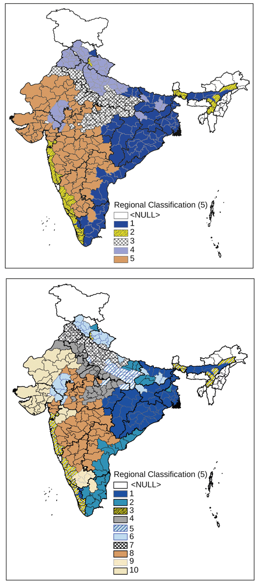
Figure 3 New typology zones derived from cluster analysis
Source: Drawn by the authors using the DLS database compiled by ICRISAT.
4.2 Characteristics of the New Typology Zones
What spatial patterns does each zone in our proposed typology show? If each zone did not show coherent patterns, our new typology would be of little value. We thus prepared Table 1, showing the characteristics of each zone as derived from the cluster analysis. It specifically reports the spatial distribution of each zone and the average values of the 16 variables on which our clustering was based. We describe the characteristics for each of the five large zones (L1–L5), with explanations for medium-level zones (M1–M10) within each large zone.
Table 1 Characteristics of new typology zones for Indian agriculture, derived from cluster analysis
| Large (5 zones) | Medium (10 zones) | Number of districts | States included* | Rainfall | Intensity, initial value | Irrigation ratio, initial value | Irrigation ratio, trend | Area under individual crop in gross cultivated area, initial value | Name (preliminary) | |||||||||||
| Annual | June | July-August | rice | wheat | maize | sorghum | pearl millet | finger millet | barley | chickpea | pigeonpea | other pulses | ||||||||
| L1 | (M1,2) | 83 | OR, WB, TN, AP, BH, CG, AS, JK, MP, UP, HP, MH | 0.20 | 0.19 | -0.11 | 0.14 | 0.30 | -0.41 | 1.02 | -0.47 | -0.28 | -0.42 | -0.31 | -0.04 | -0.19 | -0.43 | -0.41 | 0.12 | Rice zone |
| M1 | 53 | OR, WB, CG, AS, BH, JK, MP, MH | 0.42 | 0.51 | 0.25 | 0.04 | -0.26 | -0.31 | 1.18 | -0.47 | -0.17 | -0.53 | -0.38 | -0.11 | -0.23 | -0.36 | -0.38 | 0.18 | High rainfall, rainfed rice zone | |
| M2 | 30 | AP, TN, BH, UP | -0.18 | -0.37 | -0.73 | 0.30 | 1.28 | -0.59 | 0.72 | -0.48 | -0.48 | -0.22 | -0.18 | 0.08 | -0.12 | -0.55 | -0.46 | -0.01 | Low rainfall, irrigated rice zone | |
| L2 | M3 | 29 | KL, AS, MH, KN, WB | 2.43 | 2.22 | 2.14 | 0.02 | -0.18 | -0.96 | 0.77 | -0.80 | -0.38 | -0.64 | -0.51 | 0.32 | -0.50 | -0.69 | -0.58 | -0.59 | Extreme rainfall, rainfed, non-foodgrains zone |
| L3 | (=M4,5) | 48 | UP, MP, HY, RS | -0.32 | -0.49 | 0.03 | -0.10 | 0.01 | 0.96 | -0.43 | 0.86 | -0.33 | -0.11 | 0.11 | -0.26 | 1.17 | 1.65 | 1.06 | -0.20 | Semi-arid, extensive, wheat-pulse zone |
| M4 | 30 | MP, UP, HY, RS | -0.35 | -0.53 | 0.06 | -0.37 | -0.33 | 1.07 | -0.68 | 1.14 | -0.51 | 0.03 | 0.29 | -0.28 | 0.15 | 2.23 | 0.66 | -0.26 | Semi-arid, extensive, wheat-chickpea zone | |
| M5 | 18 | UP, MP | -0.28 | -0.43 | -0.03 | 0.36 | 0.57 | 0.78 | 0.00 | 0.38 | -0.03 | -0.36 | -0.18 | -0.23 | 2.86 | 0.67 | 1.73 | -0.11 | Semi-arid, extensive, pigeonpea-barley zone | |
| L4 | (=M6,7) | 61 | UP, PJ, UK, RS, HP, BH, GJ, HY | -0.33 | -0.28 | -0.14 | 1.11 | 0.54 | 0.11 | -0.40 | 0.93 | 1.29 | -0.61 | -0.26 | -0.24 | 0.14 | 0.10 | -0.32 | -0.53 | Semi-arid, intensive, maize zone |
| M6 | 27 | HP, RS, BH, GJ, UK | -0.19 | -0.07 | -0.11 | 1.34 | -0.29 | -0.56 | -0.49 | -0.01 | 1.91 | -0.58 | -0.42 | -0.20 | 0.20 | -0.29 | -0.39 | -0.56 | Semi-arid, intensive, maize-dominant zone | |
| M7 | 34 | UP, PJ, HY | -0.44 | -0.45 | -0.17 | 0.92 | 1.19 | 0.64 | -0.33 | 1.68 | 0.79 | -0.63 | -0.12 | -0.28 | 0.10 | 0.42 | -0.27 | -0.51 | Irrigation-intensive, wheat-maize zone | |
| L5 | (=M8,9,10) | 90 | MH, RS, MP, KN, GJ, AP | -0.57 | -0.44 | -0.51 | -0.83 | -0.58 | 0.10 | -0.68 | -0.40 | -0.31 | 1.07 | 0.56 | 0.24 | -0.38 | -0.33 | 0.22 | 0.55 | Rainfed, extensive, millet zone |
| M8 | 57 | MH, MP, AP, RS, KN, GJ | -0.42 | -0.31 | -0.34 | -0.83 | -0.62 | 0.17 | -0.65 | -0.30 | -0.21 | 1.73 | -0.14 | -0.18 | -0.40 | -0.18 | 0.66 | 0.40 | Rainfed, extensive, jowar zone | |
| M9 | 7 | KN | -0.50 | -0.71 | -1.20 | -0.70 | -0.11 | -0.50 | -0.31 | -0.89 | -0.52 | -0.22 | -0.39 | 5.35 | -0.54 | -0.66 | -0.06 | 1.02 | Rainfed, extensive, ragi zone | |
| M10 | 26 | RS, GJ, MH | -0.93 | -0.64 | -0.70 | -0.85 | -0.63 | 0.10 | -0.85 | -0.48 | -0.49 | -0.04 | 2.36 | -0.23 | -0.28 | -0.56 | -0.67 | 0.77 | Rainfed, extensive, bajra zone | |
Notes: 1. *Name of States: AP=Andhra Pradesh, AS=Assam, BH=Bihar,
CG=Chhattisgarh, GJ=Gujarat, HP=Himachal Pradesh, HY=Haryana, JK=Jharkhand,
KN=Karnataka, KL=Kerala, MP=Madhya Pradesh,
MH=Maharashtra, OR=Orissa, PJ=Punjab, RS=Rajasthan, TN=Tamil Nadu, UP=Uttar
Pradesh, UK=Uttarakhand, WB=West Bengal.
2. This table
reports the normalised cluster-wise average. Therefore, under the normal
distribution, the threshold for the top 5 per cent (bottom 5 per cent) is
+1.64 (-1.64), while the threshold for the top 10 per cent (bottom 10 per
cent) is +1.28 (-1.28).
Source: Drawn by the authors using the DLS database compiled by ICRISAT.
Zone L1 contains districts where rice cultivation dominated in the initial years (the “rice zone”). The rice zone (L1) is subdivided into M1 districts in States such as Orissa, West Bengal, and Assam, and M2 districts in States such as Andhra Pradesh and Tamil Nadu. The two sub-zones are distinguished by the amount of rainfall and the extent of irrigation development: M1 is thus called a “high rainfall, rainfed rice zone” while M2 is called a “low rainfall, irrigated rice zone.”
Zone L2 (=zone M3) spreads into districts in hilly and coastal areas in Kerala, Assam, coastal Andhra Pradesh, and coastal Karnataka. Due to extremely high rainfall, rice crops were dominant in the initial years as in Zone L1. However, L2 was distinguished from other zones by the relatively high extent to which non-foodgrain crops were produced. For this reason, we call L2 “extreme rainfall, rainfed, non-foodgrain zone.”
Zones L3–L5 are characterised by semi-arid agriculture, distinguished by the extent of land use intensity, irrigation ratio, and traditional crops. Using the most traditional crops in these districts as reference, we call L3 “semi-arid, extensive, wheat-pulse zone,” L4 “semi-arid, intensive, maize zone,” and L5 “rainfed, extensive, millet zone.”
Zone L3 “semi-arid, extensive, wheat-pulse zone” is further subdivided into M4 (semi-arid, extensive, wheat-chickpea zone), which spreads over Madhya Pradesh, Uttar Pradesh, Haryana, and Rajasthan, and M5 (semi-arid, extensive, pigeonpea-barley zone), which spreads over Uttar Pradesh and Madhya Pradesh. The key crop characterising M4 is chickpea (gram), while the crop characterising M5 is pigeonpea (tur/arhar).
Zone L4 (semi-arid, intensive, maize zone) is similarly subdivided into M6 (semi-arid, intensive, maize-dominant zone) and M7 (irrigation-intensive, wheat-maize zone). In M6, the importance of maize in the traditional cropping patterns was more distinct than in M7. M7 may be alternatively called “Punjab-type zone.” It contains districts in Punjab, Haryana, and western Uttar Pradesh, where the Green Revolution first spread in the late 1960s.
Zone L5 contains three sub-zones, differentiated by the most important millet crop. M8 districts, where sorghum (jowar) dominated among the millets during the initial years of our reference period, are located in Maharashtra, Madhya Pradesh, Andhra Pradesh, and Rajasthan. M9 districts, where finger millet (ragi) was the dominant millet, are only found in Karnataka. M10 districts, characterised by the importance of pearl millet (bajra) among millets, are located in Rajasthan, Gujarat, and Maharashtra.
Table 2 Changes in intensity of agricultural production and cropping patterns, by typology zone
| Large (5 zones) | Medium (10 zones) | Name (preliminary) | States included* | Indices for intensity of agric. production# | Area under individual crop in gross cultivated area# | ||||||||||||
| intensity | srw | snfg | fertilizer | rice | wheat | maize | sorghum | pearl millet | finger millet | barley | chickpea | pigeonpea | other pulses | ||||
| L1 | Rice zone | OR, WB, TN, AP, BH, CG, AS, JK, MP, UP, HP, MH | ( , , ) | (+, , ) | ( , , ) | ( , , ) | (+, , +) | ( , , ) | ( , , ) | ( , , ) | ( , , ) | ( , , ) | ( , , ) | ( , , ) | ( , , ) | ( , , ) | |
| M1 | High rainfall, rainfed rice zone | OR, WB, CG, AS, BH, JK, MP, MH | ( , , ) | (+, , ) | ( , , ) | ( , , ) | (+, , +) | ( , , ) | ( , , ) | ( , , ) | ( , , ) | ( , , ) | ( , , ) | ( , , ) | ( , , ) | ( , , ) | |
| M2 | Low rainfall, irrigated rice zone | AP, TN, BH, UP | ( , - , ) | ( , , ) | ( , , ) | (+, , ) | ( , , ) | ( , , ) | ( , , ) | ( , , ) | ( , , ) | ( , , ) | ( , , ) | ( , + , ) | ( , , ) | ( , , ) | |
| L2 | M3 | Extreme rainfall, rainfed, non-foodgrains zone | KL, AS, MH, KN, WB | ( , , ) | (+, , +) | (+, , +) | ( , , ) | ( , , ) | ( , , -) | ( , , ) | ( , , ) | ( , , ) | ( , , ) | ( , , ) | ( , , ) | ( , , ) | ( , , ) |
| L3 | Semi-arid, extensive, wheat-pulse zone | UP, MP, HY, RS | ( , , ) | ( , , ) | ( , , ) | ( , , ) | ( , , ) | (+, , +) | ( , , ) | ( , , ) | ( , , ) | ( , , ) | (+, , ) | (+, , +) | (+, , ) | ( , , ) | |
| M4 | Semi-arid, extensive, wheat-chickpea zone | MP, UP, HY, RS | ( , , ) | ( , , ) | ( , , ) | ( , , ) | ( , , ) | (+, , ) | ( , , ) | ( , , ) | ( , , ) | ( , , ) | ( , , ) | (+, , +) | ( , , ) | ( , , ) | |
| M5 | Semi-arid, extensive, pigeonpea-barley zone | UP, MP | ( , , ) | ( , , ) | ( , , ) | ( , , ) | ( , , ) | ( , , +) | ( , , ) | ( , , ) | ( , , ) | ( , , ) | (+, , ) | ( , , ) | (+, , ) | ( , , ) | |
| L4 | Semi-arid, intensive, maize zone | UP, PJ, UK, RS, HP, BH, GJ, HY | (+, , +) | ( , , ) | ( , , ) | ( , , ) | ( , , ) | (+, , +) | (+, , +) | ( , , ) | ( , , ) | ( , , ) | ( , , ) | ( , , ) | ( , , ) | ( , , ) | |
| M6 | Semi-arid, intensive, maize-dominant zone | HP, RS, BH, GJ, UK | (+, - , ) | ( , , ) | (+, , ) | ( , , ) | ( , , ) | ( , , ) | (+, , +) | ( , , ) | ( , , ) | ( , , ) | ( , , +) | ( , , ) | ( , , ) | ( , , ) | |
| M7 | Irrigation-intensive, wheat-maize zone | UP, PJ, HY | (+, + , +) | ( , , +) | ( , , ) | (+, , +) | ( , + , ) | (+, , +) | ( , , ) | ( , , ) | ( , , ) | ( , , ) | ( , , ) | ( , , ) | ( , , ) | ( , , ) | |
| L5 | Rainfed, extensive, millet zone | MH, RS, MP, KN, GJ, AP | ( , , ) | (-, , -) | ( , , ) | ( , , ) | ( , , ) | ( , , ) | ( , , ) | (+, , ) | ( , , ) | ( , , ) | ( , , ) | ( , , ) | ( , , ) | ( , , ) | |
| M8 | Rainfed, extensive, jowar zone | MH, MP, AP, RS, KN, GJ | ( , , ) | (-, , -) | ( , , ) | ( , , ) | ( , , ) | ( , , ) | ( , , ) | (+, , +) | ( , , ) | ( , , ) | ( , , ) | ( , , ) | ( , , +) | ( , , ) | |
| M9 | Rainfed, extensive, ragi zone | KN | ( , - , -) | (-, , -) | ( , , ) | (+, , ) | ( , , ) | (-, , -) | ( , , ) | ( , , ) | ( , , ) | (+, + , +) | ( , , ) | ( , , ) | ( , , ) | (+, , ) | |
| M10 | Rainfed, extensive, bajra zone | RS, GJ, MH | (-, , ) | (-, + , -) | ( , , ) | ( , + , ) | (-, , -) | ( , + , ) | ( , , ) | ( , , ) | (+, , +) | ( , , ) | ( , + , ) | ( , , ) | ( , , ) | ( , + , ) | |
Notes: 1. # (x, y, z) shows the relative positions of each
cluster in the Indian average, where x indicates the initial value, y the
trend, and z the terminal value. If the relative position is high (low) at
the 20 per cent significance level, + (-) is shown. A blank implies statistical insignificance. For instance, (+, -, ) indicates that the cluster had its
initial value higher than the Indian average but the trend was more negative
than the Indian average, resulting in insignificant difference in the terminal
value.
2. *Names of States:
AP=Andhra Pradesh, AS=Assam, BH=Bihar, CG=Chhattisgarh, GJ=Gujarat,
HP=Himachal Pradesh, HY=Haryana, JK=Jharkhand, KN=Karnataka, KL=Kerala, MP=Madhya Pradesh,
MH=Maharashtra, OR=Orissa, PJ=Punjab, RS=Rajasthan, TN=Tamil Nadu, UP=Uttar
Pradesh, UK=Uttarakhand, WB=West Bengal.
Source: Drawn by the authors using the DLS database compiled by ICRISAT.
While Table 1 shows the characteristics of each zone in the initial part of the reference period, Table 2 summarises the trends experienced in districts located in each zone and the terminal characteristics, as apparent in the 2000s. It is worth noting that the high level of land use intensity among L4 districts was maintained, and that these districts were characterised by intensive use of land at the end of the reference period. In particular, districts in M7 (Punjab-type zone) witnessed a growth rate of land use intensity and fertilizer use higher than other regions. Looking at the rice-wheat ratio (srw) or the non-foodgrain ratio (snfg), the zone-wise difference is not very substantial. An exception is the rapid increase of srw in M10 (bajra zone), reflecting the replacement of bajra by wheat as irrigation developed. In districts in M10, fertilizer use increased much faster than in other zones.
As shown above, the cluster analysis using 16 variables suggests a new spatial typology of Indian agriculture. Each zone (or sub-zone) derived through the cluster analysis was associated with its own initial conditions and changes thereafter. We conclude, therefore, that the new typology can show coherent patterns in district-level descriptive analysis.
5. Correlates of District-Level Changes in Land and Fertilizer Use
5.1 Empirical Model
Thus far in this paper, we have found that our four indicators of agricultural production intensity showed different spatial dynamics across districts and zones. The four indicators were intensity (gross cultivated area divided by net cultivated area), srw (area share of rice and wheat in the total area under foodgrain crops), snfg (areas under non-foodgrain crops divided by gross cultivated area), and fertilizer (per-acre use of chemical fertilizer, the total of N, P, and K). In this section, we estimate a parametric regression model to identify correlates of district-level changes in these variables. The objective of the regression exercise is, again, descriptive. We want to quantify the districts that experienced fast (or slow) growth with respect to the four measures. Candidates for the correlates include State boundaries, the new zones suggested in the previous section, and additional structural variables. As a by-product of the regression analysis, we can evaluate how much explanatory power our new typology has in descriptive and parametric regression exercises.
The regression model we estimate is specified as:
yit = ai + (b0 + Zibk)t + uit, (1)
where yit is one of the four indicators in district i in year t, a and b are parameters to be estimated, Zi is a vector of variables that shift trends, and uit is a zero-mean error.6
As each district is associated with different time-invariant characteristics such as weather, geography, and history, the level impact of such heterogeneity is perfectly controlled by district fixed effects, ai. After controlling for such heterogeneity, which factor explains the diversity in district-level growth rate? This is the main motivation for estimating equation (1). In other words, parameters in b are the primary interest of this section. Equation (1) can be estimated by a standard one-way fixed effect panel method. As Zi in the interaction term has no variation across time, we use district-clustered robust standard errors to evaluate the statistical significance of parameter b.
We attempt four variants with respect to the choice of Zi. First, when Zi is specified as an empty set, parameter b0 identifies the Indian average growth rates of the four indicators (Model A). We then include 18 State dummies in Zi as Model B and 9 zone dummies as Model C. In Models B and C, we use the State (zone) where the largest number of districts are located as the reference, corresponding to parameter b0. Then parameter bk shows how much faster or slower growth State (zone) k experienced relative to the reference State (zone). In Model D, we include normalised variables of initial intensity measures and exogenous technology and infrastructure variables in Zi. Then parameter b0 shows the average growth rate corresponding to a hypothetical district that had the average values of all variables in Zi while parameter bk shows the marginal impact the variable has on the growth rate.
5.2 Regression Results
Regression results are shown in Table 3. As shown in Panel A, which correspond to Model A, all four indicators showed a positive trend, statistically significant at the 1 per cent level. Land use intensity increased by 0.54 percentage points a year, srw by 0.33 percentage points, snfg by 0.25 percentage points, and fertilizer by 2.66 kg/ha per year.
Table 3 Regression results for district-level changes in agricultural production intensity
| intensity (x100) | srw (x100) | snfg (x100) | fertilizer | |||||||||
| Summary Statistics | ||||||||||||
| No. of observations# | 12,620 | 12,936 | 12,680 | 12,680 | ||||||||
| Mean (standard deviation) of the dependent variable | 126.43 | (21.95) | 52.01 | (31.21) | 32.27 | (18.45) | 55.39 | (56.14) | ||||
| Regression Results | coefficient | standard error | coefficient | standard error | coefficient | standard error | coefficient | standard error | ||||
| A. Homogeneous trends across all districts | ||||||||||||
| District fixed effects to the intercept | (Yes†) | (Yes†) | (Yes†) | (Yes†) | ||||||||
| Common trend: b0 | 0.544 | *** | 0.034 | 0.328 | *** | 0.030 | 0.254 | ** | 0.027 | 2.764 | *** | 0.104 |
| R2 | 0.829 | 0.952 | 0.799 | 0.810 | ||||||||
| R2 adjusted | 0.825 | 0.951 | 0.794 | 0.806 | ||||||||
| B. State-specific trends | ||||||||||||
| District fixed effects to the intercept | (Yes†) | (Yes†) | (Yes†) | (Yes†) | ||||||||
| Base trend: b0 (reference=UP) | 0.646 | *** | 0.054 | 0.738 | *** | 0.048 | 0.208 | *** | 0.040 | 3.592 | *** | 0.207 |
| State-specific deviation of trends: bk (k = state dummy) | ||||||||||||
| Andhra Pradesh | -0.336 | *** | 0.096 | -0.391 | *** | 0.112 | 0.223 | ** | 0.087 | 1.028 | * | 0.522 |
| Assam | 0.019 | 0.153 | -0.731 | *** | 0.049 | -0.044 | 0.049 | -2.369 | *** | 0.296 | ||
| Bihar | -0.648 | *** | 0.132 | -0.316 | *** | 0.082 | -0.504 | *** | 0.185 | -0.403 | 0.327 | |
| Chhattisgarh | -0.620 | *** | 0.077 | -0.435 | *** | 0.058 | -0.328 | *** | 0.065 | -1.935 | *** | 0.395 |
| Gujarat | -0.402 | *** | 0.078 | -0.362 | *** | 0.097 | 0.132 | 0.131 | -1.003 | *** | 0.309 | |
| Himachal Pradesh | -0.322 | *** | 0.109 | -0.590 | *** | 0.052 | -0.546 | *** | 0.139 | -2.281 | *** | 0.247 |
| Haryana | 0.509 | *** | 0.190 | 0.534 | *** | 0.152 | 0.143 | 0.136 | 1.102 | * | 0.612 | |
| Jharkhand | -0.582 | *** | 0.088 | -0.575 | *** | 0.071 | 0.142 | ** | 0.069 | -1.934 | *** | 0.328 |
| Karnataka | -0.210 | ** | 0.098 | -0.678 | *** | 0.087 | -0.070 | 0.096 | -0.719 | * | 0.399 | |
| Kerala | -0.499 | *** | 0.187 | -0.708 | *** | 0.060 | 0.415 | *** | 0.085 | -1.843 | *** | 0.300 |
| Maharashtra | -0.038 | 0.110 | -0.663 | *** | 0.065 | 0.190 | *** | 0.064 | -1.258 | *** | 0.258 | |
| Madhya Pradesh | 0.100 | 0.099 | -0.546 | *** | 0.086 | 0.203 | ** | 0.098 | -2.113 | *** | 0.241 | |
| Orissa | 0.106 | 0.093 | -1.030 | *** | 0.069 | -0.127 | * | 0.065 | -2.318 | *** | 0.289 | |
| Punjab | 0.809 | *** | 0.142 | 0.088 | 0.112 | -0.538 | *** | 0.066 | 1.020 | *** | 0.244 | |
| Rajasthan | -0.115 | 0.091 | -0.474 | *** | 0.088 | 0.245 | ** | 0.095 | -2.411 | *** | 0.287 | |
| Tamil Nadu | -0.779 | *** | 0.087 | -0.723 | *** | 0.096 | 0.068 | 0.103 | 0.399 | 0.406 | ||
| Uttarakhand | -0.626 | *** | 0.154 | -0.818 | *** | 0.088 | -1.596 | *** | 0.523 | -0.733 | 1.850 | |
| West Bengal | 0.881 | *** | 0.173 | -0.510 | *** | 0.074 | 0.225 | *** | 0.051 | 0.082 | 0.313 | |
| R2 | 0.871 | 0.969 | 0.827 | 0.873 | ||||||||
| R2 adjusted | 0.867 | 0.968 | 0.822 | 0.870 | ||||||||
| F (18,310) stat for bk=0 for all k. | 20.08 | *** | 28.66 | *** | 17.47 | *** | 37.48 | *** | ||||
| C. Typology-zone-specific trends (10 zones) | ||||||||||||
| District fixed effects to the intercept | (Yes†) | (Yes†) | (Yes†) | (Yes†) | ||||||||
| Base trend: b0 (reference=8. jowar zone) | 0.584 | *** | 0.057 | 0.188 | *** | 0.045 | 0.407 | *** | 0.059 | 2.526 | *** | 0.177 |
| Zone-specific deviation of trends: bk (k = cluster dummy) | ||||||||||||
| 1. High rainfall, rainfed rice zone | -0.003 | 0.121 | -0.075 | 0.065 | -0.300 | *** | 0.077 | -0.372 | 0.254 | |||
| 2. Low rainfall, irrigated rice zone | -0.451 | *** | 0.103 | 0.087 | 0.084 | -0.300 | ** | 0.118 | 1.972 | *** | 0.318 | |
| 3. Ext. rainfall, rainfed, non-fg zone | -0.163 | 0.169 | -0.099 | 0.063 | 0.047 | 0.078 | -0.228 | 0.329 | ||||
| 4. Semi-arid, extensive, wheat-chickpea zone | 0.224 | * | 0.117 | 0.327 | ** | 0.156 | 0.049 | 0.086 | -0.247 | 0.314 | ||
| 5. Semi-arid, extensive, pigeonpea-barley zone | 0.121 | 0.085 | 0.779 | *** | 0.075 | -0.411 | *** | 0.079 | 0.523 | 0.356 | ||
| 6. Semi-arid, intensive, maize zone | -0.366 | *** | 0.093 | 0.068 | 0.095 | -0.722 | *** | 0.124 | -0.426 | 0.337 | ||
| 7. Punjab type zone | 0.373 | *** | 0.128 | 0.578 | *** | 0.065 | -0.330 | *** | 0.092 | 2.037 | *** | 0.276 |
| 9. Rainfed, extensive, ragi zone | -0.357 | *** | 0.081 | -0.114 | 0.094 | 0.142 | 0.088 | 0.650 | 0.498 | |||
| 10. Rainfed, extensive, bajra zone | -0.194 | ** | 0.086 | 0.009 | 0.070 | 0.039 | 0.089 | -0.979 | *** | 0.307 | ||
| R2 | 0.845 | 0.962 | 0.818 | 0.855 | ||||||||
| R2 adjusted | 0.841 | 0.961 | 0.813 | 0.851 | ||||||||
| F (9, 310) stat for bk=0 for all k. | 10.53 | *** | 31.06 | *** | 14.52 | *** | 20.08 | *** | ||||
Table 3 Regression results for district-level changes in agricultural production intensity (continued)
| intensity (x100) | srw (x100) | snfg (x100) | fertilizer | |||||||||
| coefficient | standard error | coefficient | standard error | coefficient | standard error | coefficient | standard error | |||||
| D. Initial-Factor-Dependent Trends | ||||||||||||
| District fixed effects to the intercept | (Yes†) | (Yes†) | (Yes†) | (Yes†) | ||||||||
| Base trend: b0 | 0.530 | *** | 0.048 | 0.339 | *** | 0.030 | 0.257 | *** | 0.032 | 2.658 | *** | 0.102 |
| Deviation for the following variables: bk (k = structural factors) | ||||||||||||
| intensity, initial (normalised) | -0.109 | 0.072 | 0.113 | *** | 0.031 | -0.207 | *** | 0.051 | -0.017 | 0.091 | ||
| iratio, initial (normalised) | 0.181 | ** | 0.078 | 0.251 | *** | 0.043 | 0.102 | ** | 0.046 | 0.485 | *** | 0.114 |
| iratio, trend (normalised) | 0.224 | *** | 0.043 | 0.220 | *** | 0.025 | 0.101 | *** | 0.029 | 0.478 | *** | 0.073 |
| srw, initial (normalised) | 0.085 | 0.056 | -0.113 | *** | 0.036 | -0.178 | *** | 0.038 | -0.130 | 0.103 | ||
| snfg, initial (normalised) | -0.005 | 0.048 | -0.001 | 0.035 | -0.053 | 0.039 | -0.174 | ** | 0.084 | |||
| fertilizer, initial (normalised) | -0.136 | ** | 0.052 | -0.102 | *** | 0.035 | 0.019 | 0.030 | 0.946 | *** | 0.119 | |
| rainfall, 42 year average (norm.) | -0.030 | 0.065 | -0.017 | 0.039 | 0.227 | *** | 0.038 | -0.001 | 0.145 | |||
| road density, initial (norm.) | -0.078 | 0.148 | 0.074 | 0.075 | -0.076 | 0.075 | 0.714 | ** | 0.319 | |||
| market density, initial (norm.) | 0.169 | *** | 0.063 | 0.041 | 0.033 | -0.014 | 0.035 | 0.031 | 0.169 | |||
| dummy for missing market info | 0.008 | 0.064 | -0.079 | * | 0.042 | -0.081 | 0.056 | 0.273 | * | 0.142 | ||
| R2 | 0.844 | 0.966 | 0.818 | 0.877 | ||||||||
| R2 adjusted | 0.840 | 0.965 | 0.813 | 0.874 | ||||||||
| F( 10, 310) stat for bk=0 for all k. | 6.43 | *** | 20.73 | *** | 6.64 | *** | 27.62 | *** | ||||
Notes: 1. Estimated by weighted least squares with district-clustered robust standard errors. The weights are: NCA for intensity, the total foodgrain area for srw, gca for snfg, and gca for fertilizer. ***: Statistically significant at 1 per cent, **: statistically significant at 5 per cent, and *: statistically significant at 10 per cent. See Table 1 for the distribution of districts across 10 zones used in Panel C. The summary statistics for original variables used to calculate shifters in Panel D are available on request from the authors.
† For brevity, district fixed effects on intercepts are not reported.
They are jointly significant at the 0.1 per cent level in all specifications.
# Although we potentially use 13,062 observations (=311 districts x 42 years), the
actual number of observations used in regressions was less than this due to
missing observations.
Names of States:
AP=Andhra Pradesh, AS=Assam, BH=Bihar, CG=Chhattisgarh, GJ=Gujarat,
HP=Himachal Pradesh, HY=Haryana, JK=Jharkhand, KN=Karnataka, KL=Kerala,MP=Madhya Pradesh,
MH=Maharashtra, OR=Orissa, PJ=Punjab, RS=Rajasthan, TN=Tamil Nadu, UP=Uttar
Pradesh, UK=Uttarakhand, WB=West Bengal.
Source: Drawn by the authors using the DLS database compiled by ICRISAT.
Panel B in Table 3 shows the regression results when each State was allowed to have a different growth rate. As the number of districts in Uttar Pradesh (UP) was the largest, we used UP as the reference State. The null hypothesis of homogeneous growth rates across States was rejected at the 1 per cent level, as shown in the last row of Panel B. Land use intensity (intensity) grew faster than UP in districts in West Bengal, Punjab, and Haryana, while it grew slower by more than 0.5 percentage points in districts in Tamil Nadu, Bihar, Chhattisgarh, Uttarakhand, and Jharkhand. In Punjab and Haryana, where intensity grew faster, districts also witnessed faster growth in fertilizer. The importance of non-foodgrain crops (snfg) increased faster than UP in districts in Maharashtra, Rajasthan, West Bengal, and Andhra Pradesh. Using estimates for b0 and bk in Panel B, we examined the States that showed a dynamic change that was most similar to the one found at the national level (Panel A). Interestingly, all 19 States had one or more variables out of the four that was associated with a statistically-significant difference from the national average. In this sense, no State in India represents the Indian average. In a relative sense, however, we found that the dynamic changes observed in Gujarat, followed by Karnataka and Maharashtra, were the most similar to the national pattern.
Panel C in Table 3 shows the regression result when each zone in Table 1 was allowed to have a different growth rate. As the number of districts in M8 (rainfed, extensive, jowar zone) is the largest, we used the jowar zone as the reference zone. The null hypothesis of homogeneous growth rates across zones was, again, rejected at the 1 per cent level. The variable intensity grew at the fastest rate in districts belonging to M7 (Punjab-type zone), followed by districts belonging to M4 (semi-arid, extensive, wheat-chickpea zone). In contrast, density grew at significantly lower rates in M9 (ragi zone) and M10 (bajra zone). A similar contrast was found for srw, snfg, and fertilizer. Although using a much smaller number of explanatory variables, Model C explained the variation in data as well as Model B did, as shown by the adjusted R2 reported in Table 3. We therefore judge the ten-zone typology shown in Figure 3 as being fairly useful. This does not imply that there will be other typologies that have a higher R2 than model C and a smaller number of zones. The point here is that our typology, which was derived using the criterion of utilising the information on initial conditions and trends in irrigation only, has reasonable explanatory power in parametric models for spatial changes when we compare it with other existing typologies.7
Finally, Model D employs structural factors as shifters of heterogeneous growth rates. In other words, this is an attempt to open the black box represented by State- or zone-specific growth rates by borrowing insights from microeconomic theory explained in the introduction. We utilised information contained in 8 variables as structural shifters: intensity (initial value8); irrigation ratio, denoted by iratio (initial and trend); srw (initial); snfg (initial); fertilizer (initial); rainfall (42 year average); road density (initial), and market density (initial and dummy for missing information).9 The null hypothesis of homogeneous growth rates regardless of the structural factors was rejected at the 1 per cent level. The regression results (Panel D, Table 3) clearly show that both the initial level and trend of iratio were the most important determinants of heterogeneous growth rates in intensity, srw, snfg, and fertilizer. The initial level of road density was associated with a higher growth rate of fertilizer, while the initial level of market density was associated with a higher growth rate of intensity. Therefore, the disparity in infrastructure development during the 1960s resulted in disparity in agricultural intensification after that period. Furthermore, the spatial dynamics of srw and snfg, which show different aspects of commercialisation of agriculture, were diverse across districts, reflecting the difference in the initial conditions with respect to cropping and rainfall patterns. Many of the coefficients on these variables had opposite signs as between srw and snfg. The adjusted R2 for Model D was similar to the one for Model C, implying that the ten-zone typology has an explanatory power as high as a structural model.
6. Conclusion
In this paper, we described spatial patterns of long-term changes in Indian agriculture at the district level, using a balanced panel dataset that covered the period from 1965-6 to 2006-7 (42 years). The main findings from our investigation of land use intensity, the ratio of rice and wheat in areas under foodgrain, the ratio of non-foodgrain in gross cultivated area, fertilizer use intensity, and individual crop shares in gross cultivated areas, were as follows.
First, there was huge heterogeneity across districts in the speed of agricultural intensification over the last 42 years. Secondly, the eyeball perusal of GIS maps identified, among other changes, a shift of rice production into the interior districts of north India, a shift of wheat production eastwards in north India, the appearance of maize production centres in the interior districts of the Deccan, and a southward shift in chickpea production. The spatial shift appeared consistent with the comparative advantages that characterised each district. Thirdly, we attempted to aggregate districts into zones using cluster analysis based similarities with respect to rainfall, initial cropping and land-use patterns, and initial conditions and changes in irrigation. The proposed classification showed reasonable explanatory power in describing spatial patterns of long-term changes at the district level. Fourthly, we estimated a parametric regression model to identify correlates that were associated with heterogeneous growth rates of land use intensity, the share of rice and wheat in foodgrains, the share of non-foodgrains in gross cultivated area, and fertilizer use intensity across districts. The results confirmed the critical role of irrigation, market, and road development in facilitating the intensification of agricultural production. The regression results also clarified the different aspects of agricultural commercialisation represented by the rice-wheat share and the foodgrain share. These findings have enriched our knowledge of spatial aspects of agricultural development in India.
The analysis in this paper is, however, descriptive and preliminary in nature. Quantifying the contribution of spatial changes to aggregate productivity improvement is a matter for further study. More fundamental determinants of infrastructure and market development need to be examined in historical, institutional, and spatial context; this task, too, is left for further research. In the current paper, infrastructure and market development, including the key input of irrigation, were regarded as exogenous to farmers’ decision-making. Considering the political economy context in which development occurs, this is unsatisfactory. Another area for future work is more disaggregated analysis that combines household and village-level changes in cropping pattern with changes at the district or State (zone) levels. It is possible that the same change at the district level is observed in two districts despite within-district, inter-village changes being substantially different in the two districts. Such cases will shed further light to our understanding of the interaction between market development and agricultural production. Extending the analysis to include more recent years is also a task for further research.
Acknowledgements: We thank V. K. Ramachandran, Yoshifumi Usami, Haruka Yanagisawa, participants at the Tenth Anniversary Conference of the Foundation for Agrarian Studies, participants at the TINDAS (Tokyo Centre for the Contemporary India Area Studies Project) workshops, and two anonymous referees of this journal for their useful comments on earlier versions of this paper. We are also grateful to M. C. S. Bantilan, P. Parthasarathy Rao, and E. Jagadeesh for providing us with the DLS data.
Notes
1 See de Janvry et al. (1991) for how shadow prices are defined in mathematical models of farmers facing underdeveloped markets.
3 The dataset includes crop information for oilseeds, sugarcane, cotton, potato, onion, and fodder crops. In this paper, we aggregate them as non-foodgrain crops. Crop-wise analysis of non-foodgrain crops is left for further analysis.
4 Figure 2 was redrawn using the sub-sample of the period up to 1995. The redrawn figure shows more compact distribution for snfg and srw. The redrawn figure is available on request from the authors.
5 Specifically, we adopt a hierarchical clustering algorithm based on Ward method using similarity of Euclid and the same weight for observable variables (standardised) in calculating the similarities. See Everitt et al. (2001) for methodological details. The command cluster in the STATA 10 software was used to obtain clustering results.
6 Equation (1) has its dependent variable in levels, not in their logs, and is estimated by weighted least squares (WLS). This is because the motivation for the regression analysis is descriptive, i.e., to obtain conditional means of district-level variables (intensity, srw, snfg, and fertilizer) that are aggregated consistently to the national average. By applying WLS to level variables with proper weights (nca for intensity, the total foodgrain area for srw, gca for snfg, and gca for fertilizer), we can achieve this consistent aggregation. Furthermore, three of the four dependent variables are already in ratios (multiplied by 100), so that the coefficient estimates on the time trend have an intuitive meaning, that of average annual changes in percentage points. Regarding the fourth variable, fertilizer, it may be a good idea to take logs. However, the results are very similar when we use logs (full results are available on request from the authors).
7 In this paper, we compare our new typology (Panel C) and state boundaries (Panel B). We also estimated a similar model using the 18-zone typology of Rao et al. (2004). Adjusted R2 was 0.850 (intensity), 0.957 (srw), 0.810 (snfg), and 0.847 (fertilizer) (full results are available from the authors on request). These numbers are comparable to those reported in Panel C, Table 3. In this comparison as well, our new typology shows reasonable explanatory power in describing the spatial patterns.
9 We use the per-acre density of principal and sub-markets in a district. As this information was missing for many districts in the early years in Orissa, Bihar, and West Bengal, we included a dummy for the data missing as a shifter of growth rates.
References
| Bhalla, G. S., and Singh, G. (2001), Indian Agriculture: Four Decades of Development, New Delhi: Sage Publications. | |
| Bhalla, G. S., and G. Singh, G. (2009), “Economic Liberalisation and Indian Agriculture: A Statewise Analysis,” Economic and Political Weekly, vol. 46, no. 52, pp. 34-44. | |
| Bhalla, G. S., and G. Singh, G. (2012), Economic Liberalisation and Indian Agriculture: A District-Level Study, Sage Publications, New Delhi. | |
| Bhalla, G. S., and Tyagi, D. S. (1989), Patterns in Indian Agricultural Development: A District Level Study, Institute for Studies in Industrial Development, New Delhi. | |
| de Janvry, A., Fafchamps, M, and Sadoulet, E. (1991), “Peasant Household Behaviour with Missing Markets: Some Paradoxes Explained,” Economic Journal , vol. 101, no. 409, pp. 1400-17. | |
| Everitt, B. S., Landau, S., and Leese, M. (2001), Cluster Analysis, Arnold, London, 4th ed. | |
| ICRISAT (International Crops Research Institute for the Semi-Arid Tropics) (1998), District Level Database Documentation — 13 States of India, Volume I: Documentation of Files: 1966-94 Database (1966 district boundaries), ICRISAT, Patancheru. | |
| ICRISAT (International Crops Research Institute for the Semi-Arid Tropics) (1999), Typology Construction and Economic Policy Analysis for Sustainable Rainfed Agriculture ICRISAT, Patancheru. | |
| Kurosaki, T. (1999), “Agriculture in India and Pakistan, 1900-95: Productivity and Crop Mix,” Economic and Political Weekly, vol. 34, no. 52, pp. A160-8, Dec 25. | |
| Kurosaki, T. (2002), “Agriculture in India and Pakistan, 1900-95: A Further Note,” Economic and Political Weekly, vol. 37, no. 30, pp. 3149-52, Jul 27. | |
| Kurosaki, T. (2003), “Specialisation and Diversification in Agricultural Transformation: The Case of West Punjab, 1903-1992,” American Journal of Agricultural Economics, vol. 85, no. 2, pp. 373-87. | |
| Kurosaki, T. (2011), “Compilation of Agricultural Production Data in Areas Currently in India, Pakistan, and Bangladesh from 1901/02 to 2001/02,” G-COE discussion paper, no.169/ PRIMCED discussion paper, no. 6, Hitotsubashi University, Tokyo, Feb. | |
| Kurosaki, T. (2015), “Long-Term Agricultural Growth in India, Pakistan, and Bangladesh from 1901/2 to 2001/2,” International Journal of South Asian Studies, volume 7, pp. 61–86 (forthcoming). | |
| Rao, Parthasarathy P., Birthal, P. S., Kar, Dharmendra, Wickramaratne, S. H. G., and Shrestha, H. R. (2004), Increasing Livestock Productivity in Mixed Crop-Livestock Systems in South Asia, ICRISAT, Patancheru. | |
| Takayama, A., and Judge, G. (1971), Spatial and Temporal Price and Allocation Models, North Holland Publishing, Amsterdam. | |
| Thorner, D. (1996), Ecological and Agrarian Regions of South Asia circa 1930, Oxford University Press, Karachi. | |
| Timmer, C. P. (1997), “Farmers and Markets: The Political Economy of New Paradigms,” American Journal of Agricultural Economics, vol. 79, no. 2, pp. 621-7. |
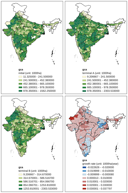
Appendix Map 1 District-level changes, gross cultivated area (1965-2007)
Source: Drawn by the authors using the DLS database compiled by ICRISAT.
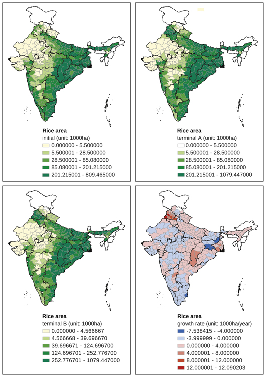
Appendix Map 2 District-level changes, rice area (1965–2007)
Source: Drawn by the authors using the DLS database compiled by ICRISAT.
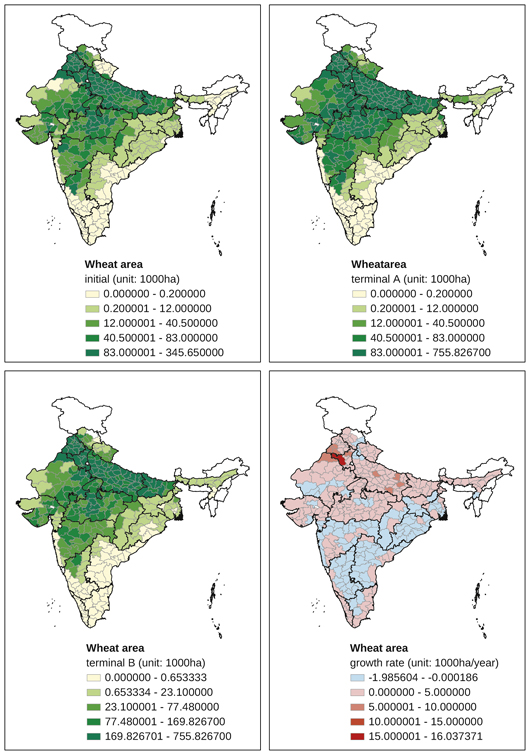
Appendix Map 3 District-level changes, wheat area (1965–2007)
Source: Drawn by the authors using the DLS database compiled by ICRISAT.
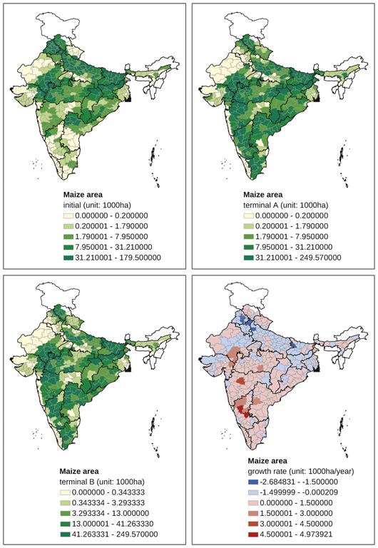
Appendix Map 4 District-level changes, maize area (1965–2007)
Source: Drawn by the authors using the DLS database compiled by ICRISAT.
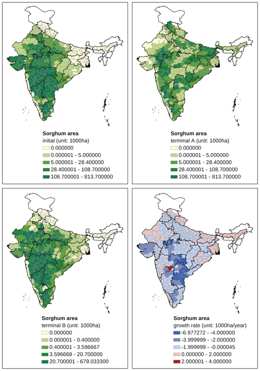
Appendix Map 5 District-level changes, sorghum area (1965–2007)
Source: Drawn by the authors using the DLS database compiled by ICRISAT.
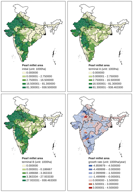
Appendix Map 6 District-level changes, pearl millet area (1965–2007)
Source: Drawn by the authors using the DLS database compiled by ICRISAT.
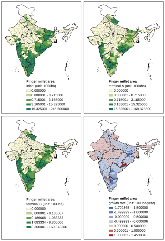
Appendix Map 7 District-level changes, finger millet area (1965–2007)
Source: Drawn by the authors using the DLS database compiled by ICRISAT.
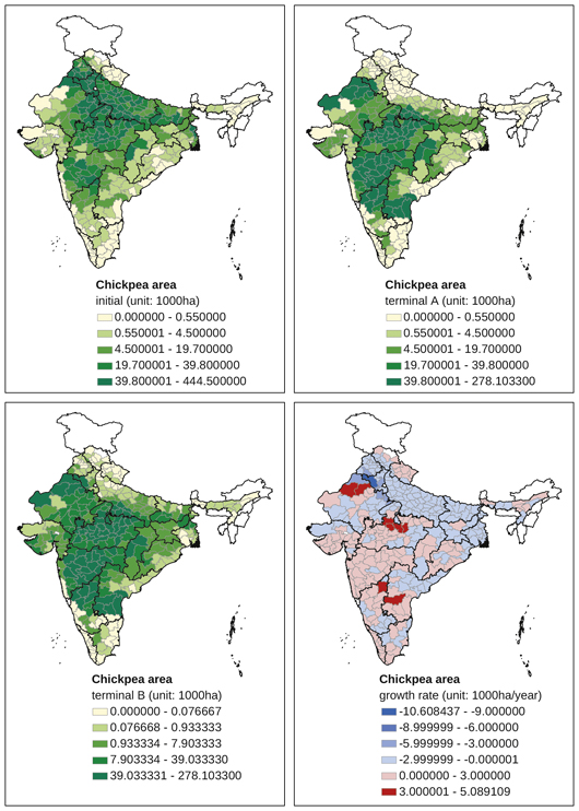
Appendix Map 8 District-level changes, chickpea area (1965–2007)
Source: Drawn by the authors using the DLS database compiled by ICRISAT.
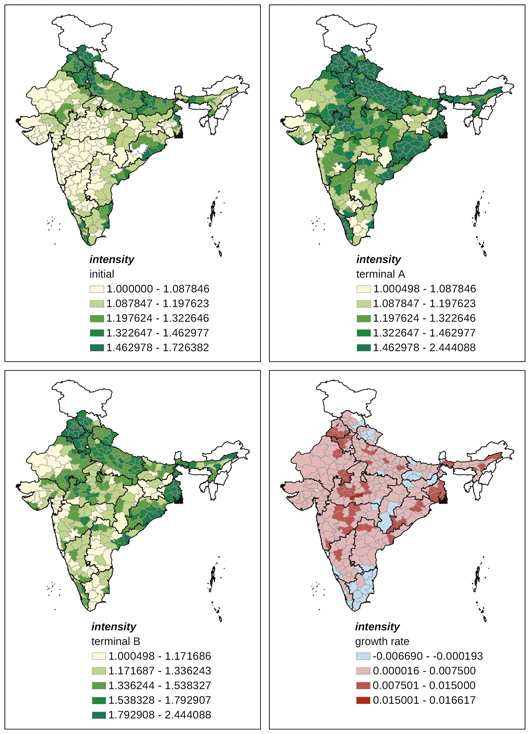
Appendix Map 9 District-level changes, intensity (=gca/net cultivated area) (1965–2007)
Source: Drawn by the authors using the DLS database compiled by ICRISAT.
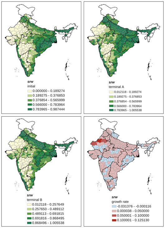
Appendix Map 10 District-level changes, srw (share of rice and wheat area in foodgrain area) (1965–2007)
Source: Drawn by the authors using the DLS database compiled by ICRISAT.
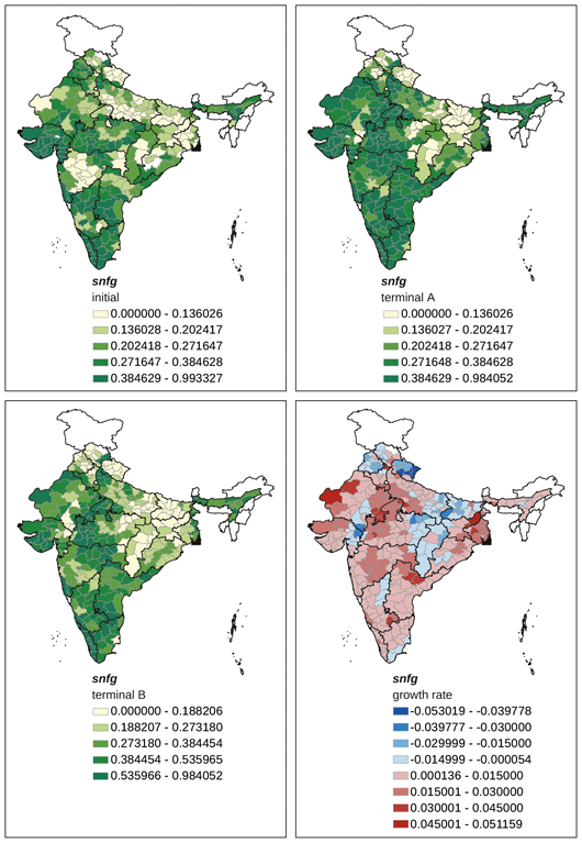
Appendix Map 11 District-level changes, snfg (= share of non-foodgrain crops area in gca) (1965–2007)
Source: Drawn by the authors using the DLS database compiled by ICRISAT.


